Competing Risk Forecasts¶

FIFE can be used to forecast time-to-event under a competing risks framework. Competing risks analysis is useful when you desire to predict not only when a terminal event occurs, but which terminal event occurs. Forecasts from the survival modeler and the exit modeler can be combined to produce cumulative incidence function and cause-specific hazard forecasts. An alternative approach is to model the subdistribution of risk, which is not currently implemented in FIFE (Schmid and Berger, 2020).

Suppose there are \(M\) different terminal events that occur at times \(T_{i1}, T_{i2}, ..., T_{iM}\) for individual \(i\), where each terminal event time shares a common individual-specific time scale and starting period of 0. The period of analysis terminates at \(T_{i0}\), representing an individual-specific right-censoring time. Note, all individuals share the same right-censoring absolute time, which is the last observed time period in the data.

For each individual we only observe the first occurring event, \(T_i=min(T_{i0},T_{i1}, T_{i2}, ..., T_{iM})\), and which event occurred, \(d_i=\underset{d\in\{0,1,2,...,M\}}{argmin}T_{id}\). After time \(T_i\), individual \(i\) is no longer observed in the data.

It is assumed that if censoring and a terminal event occur at the same time then only censoring is observed. This is because a terminal event can only be verified in period \(T_i + 1\) and censoring occurs in the last time period in the data. Additionally, it is assumed that terminal events are mutually exclusive. In other words, no two events can be simultaneously observed as a terminal event for the same individual. Thus, \(d_i\) is a singleton for every individual.

Dataset for training and prediction¶

The dataset format is similar to the one used in the single-risk case (with LGBSurvivalModeler) except that a column containing the type of terminal event for the individual must be provided as an argument to exit_col in LGBExitModeler. Currently, exit modeling is only supported for LightGBM.

We use the Rulers, Elections, and Irregular Governance dataset (REIGN) dataset (also used in this notebook) as an example for predicting not just when a leader’s reign will end but how their reign will end. The reign can end by the government type remaining the same (e.g., remains as presidential democracy, USA 2016), government type changing (e.g., changes from personal dictatorship to warlordism, Yemen 2015), or a complete country dissolution (e.g., Yugoslavia 1991).

from fife.lgb_modelers import LGBSurvivalModeler
from fife.lgb_modelers import LGBExitModeler
from fife.processors import PanelDataProcessor
from fife.utils import make_results_reproducible, plot_shap_values
from pandas import concat, date_range, read_csv, to_datetime, Index, DataFrame
from numpy import array, repeat, nan

# import warnings
#warnings.filterwarnings('ignore')

SEED = 9999
make_results_reproducible(SEED)

data = read_csv("https://www.dl.dropboxusercontent.com/s/3tdswu2jfgwp4xw/REIGN_2020_7.csv?dl=0")

# Define individual and time units
data["country-leader"] = data["country"] + ": " + data["leader"]
data["year-month"] = data["year"].astype(int).astype(str) + data["month"].astype(int).astype(str).str.zfill(2)
data["year-month"] = to_datetime(data["year-month"], format="%Y%m")
data = concat([data[["country-leader", "year-month"]],
               data.drop(["ccode", "country-leader", "leader", "year-month"],
                         axis=1)], axis=1)

data = data.drop_duplicates(["country-leader", "year-month"], keep="first")

# Process data for model input
data_processor = PanelDataProcessor(data=data, config={'NUMERIC_SUFFIXES':  ['year','month','age','tenure_months','lastelection','loss','irregular','prev_conflict','precip','couprisk','pctile_risk']})
data_processor.build_processed_data()

mdata = data_processor.data.copy()

The REIGN data does not natively come with columns indicating the type of terminal event, thus such a column needs to be engineered. In doing do so there are several notes the user should be aware of. First, the terminal event type column must be a categorical data type. Second, FIFE only uses the terminal event value from each individual’s last observation; any preceding terminal event values for the same individual are ignored. Third, FIFE’s .build_processed_data() identifies unique individuals by their spells (i.e., broken panels). That is, if an individual leaves the dataset and re-enters, they are treated as two different individuals. Therefore, terminal event types need to be provided at the last time period for each individual-spell. This can be accomplished using the _period column output with .build_processed_data() as shown below.

# Assign unique ID based off broken panels
gaps = mdata.groupby("country-leader")["_period"].shift() < mdata["_period"] - 1
spells = gaps.groupby(mdata["country-leader"]).cumsum()
mdata['country-leader-spell'] = mdata['country-leader'] + array(spells, dtype = 'str')

# Create exit status for dissolution, change of government type, and same government type
mdata['outcome'] = "Same government type"

for i in mdata['country-leader-spell'].unique():
    # Boolean index for the unique country-leader-spell observations
    dex1 = mdata['country-leader-spell'] == i
    # Boolean index for the last observation for the country-leader-spell observations
    dex2 = dex1 & (mdata['year-month'] == mdata.loc[dex1,'year-month'].max())
    # Boolean index for the last observation for the country-leader-spell observations unless it is censored
    dex3 = dex2 & (mdata['year-month'] != mdata['year-month'].max())
    # Only assign exit status if not censored
    if dex3.sum() > 0:
        futuredex = (mdata['year-month'] >= mdata.loc[dex3,'year-month'].values[0]) & (mdata['country'] == mdata.loc[dex3,"country"].values[0]) & ~dex1
        if futuredex.sum() == 0:
            mdata.loc[dex2,'outcome'] = "Dissolution" # could alternatively use dex1
        else:
            oldgovernment = mdata.loc[dex3,'government'].values[0]
            futuremdata = mdata[futuredex]
            newgovernment = futuremdata.loc[futuremdata['year-month'] == futuremdata['year-month'].min(),'government'].values[0]
            if oldgovernment == newgovernment:
                mdata.loc[dex2,'outcome'] = "Same government type" # could alternatively use dex1
            else:
                mdata.loc[dex2,'outcome'] = "Change of government type" # could alternatively use dex1

# The outcome variable must be a category type
mdata['outcome'] = mdata['outcome'].astype('category')

We can do additional feature engineering such as including features that count the number of new leaders and changes of government types in the last 10 and 20 years.

# Feature engineering (optional)
# Include number of new leaders in last 10 and 20 years
# Include number of new governments types in last 10 and 20 years
mdata['new_leader_10'] = nan
mdata['new_leader_20'] = nan
mdata['new_govt_10'] = nan
mdata['new_govt_20'] = nan

for i in mdata['country'].unique():
    dex4 = mdata['country'] == i
    for j in mdata.loc[dex4,'year'].unique():
        if mdata.loc[dex4,'year'].min() <= j - 10:
           mdata.loc[dex4 & (mdata['year'] == j), 'new_leader_10'] = mdata.loc[dex4 & (mdata['year'] >= j - 10) & (mdata['year'] < j), 'country-leader-spell'].nunique()
           mdata.loc[dex4 & (mdata['year'] == j), 'new_govt_10'] = mdata.loc[dex4 & (mdata['year'] >= j - 10) & (mdata['year'] < j), 'government'].nunique()
           if mdata.loc[dex4,'year'].min() <= j - 20:
               mdata.loc[dex4 & (mdata['year'] == j), 'new_leader_20'] = mdata.loc[dex4 & (mdata['year'] >= j - 20) & (mdata['year'] < j), 'country-leader-spell'].nunique()
               mdata.loc[dex4 & (mdata['year'] == j), 'new_govt_20'] = mdata.loc[dex4 & (mdata['year'] >= j - 20) & (mdata['year'] < j), 'government'].nunique()

# We no longer need country-leader-spell
mdata = mdata.drop(['country-leader-spell'], axis = 1)

Training and forecasting¶

Survival probabilities¶

Now that the data are prepared, we can train and forecast with the survival modeler, LGBSurvivalModeler, to obtain the survival probabilities. The survival probabilities are the probability of surviving at least up to some future time horizon and are defined to be

\[Pr(T_i\geq t|X_{i{\tau}}),\]

where \(X_{i{\tau}}\) is a vector of feature values for individual \(i\) at time \(\tau\).

Forecasts are produced for censored individuals with .forecast() up to the furthest observed time period after the initial period, \(t\in\{T_{i0}+1, T_{i0}+2, ..., T_{i0} + \check{T}\}\), where \(\check{T}=\underset{i}{max}\; T_{i}\). The features used are from the last observed row, \(X_{i} = X_{i{\tau}}=X_{i{T_{i0}}}\). Thus forecasted probabilities for all future periods for a given individual are conditional on the same observed features and are coherent up to numerical accuracy (i.e., probabilities are theoretically valid, but when summed over the full support there may be a small numerical difference from 1). Note, if a terminal event type column is in the data, it should not be passed to LGBSurvivalModeler.

# Obtain the survival probability
survival_modeler = LGBSurvivalModeler(data=mdata.drop('outcome', axis = 1))
survival_modeler.build_model(parallelize=False)
survival_modeler_forecasts = survival_modeler.forecast()

# Set custom column names
custom_forecast_headers = date_range(data["year-month"].max(),
                                      periods=len(survival_modeler_forecasts .columns)+1,
                                      freq="M").strftime("%b %Y")[1:]
survival_modeler_forecasts.columns = custom_forecast_headers
survival_modeler_forecasts

country-leader	Aug 2020	Sep 2020	Oct 2020	Nov 2020	…	Jun 2040	Jul 2040	Aug 2040	Sep 2040
Afghanistan: Ashraf Ghani	0.986044	0.965914	0.953822	0.942614	…	0.000322	0.000320	0.000273	0.000271
Albania: Rama	0.992290	0.984483	0.977156	0.968703	…	0.008364	0.008308	0.008252	0.008197
Algeria: Tebboune	0.991351	0.977605	0.965622	0.941865	…	0.007509	0.007316	0.006988	0.006939
Andorra: Espot Zamora	0.990101	0.981595	0.975345	0.966500	…	0.000727	0.000723	0.000718	0.000713
Angola: Lourenco	0.985230	0.972513	0.959758	0.947597	…	0.025139	0.024493	0.023396	0.023232
…	…	…	…	…	…	…	…	…	…
Venezuela: Nicolas Maduro	0.993150	0.986412	0.982183	0.975254	…	0.000331	0.000329	0.000321	0.000313
Vietnam: Phu Trong	0.991983	0.982679	0.968412	0.959021	…	0.002620	0.002586	0.002209	0.002123
Yemen: Houthi	0.992832	0.983635	0.950930	0.939746	…	0.056119	0.055744	0.055367	0.054997
Zambia: Lungu	0.993150	0.986317	0.981646	0.973240	…	0.008273	0.006682	0.005709	0.005411
Zimbabwe: Mnangagwa	0.993150	0.986421	0.981954	0.974727	…	0.058133	0.057746	0.057357	0.056975

Type of terminal event probabilities¶

The same data can be used to train and forecast with the exit modeler, LGBExitModeler, where the terminal event type column name is passed as an argument to exit_col. The exit modeler produces estimates for the type of terminal event, conditional on \(t\) being the last period observed. This is defined formally as

\[Pr(D_i=d|T_i= t,X_{i{\tau}}).\]

Like LGBSurvivalModeler, LGBExitModeler produces forecasts for every indvidual who is censored using features from the last observed row. Also like LGBSurvivalModeler, LGBExitModeler trains a separate model for each number of periods into the future. Unlike LGBSurvivalModeler, LGBExitModeler trains each model only on observations with an observed terminal event \(t\) periods into the future.

# Obtain the probability of type of terminal event conditional on exit that period
exit_modeler = LGBExitModeler(data=mdata, exit_col = 'outcome')
exit_modeler.build_model(parallelize=False)
exit_modeler_forecasts = exit_modeler.forecast()

# Set MultiIndex and column names
exit_modeler_forecasts = exit_modeler_forecasts.set_index('Future outcome', append = True, drop = True)
exit_modeler_forecasts = exit_modeler_forecasts.reindex(['Same government type','Change of government type','Dissolution'], axis=0,level=1)
exit_modeler_forecasts.columns = custom_forecast_headers
exit_modeler_forecasts

country-leader	Future outcome	Aug 2020	Sep 2020	…	Aug 2040	Sep 2040
Afghanistan: Ashraf Ghani	Same government type	0.805657	0.786539	…	7.802002e-01	7.515268e-01
	Change of government type	0.193860	0.212768	…	2.197998e-01	2.484732e-01
	Dissolution	0.000483	0.000693	…	9.222983e-16	9.787801e-16
Albania: Rama	Same government type	0.979288	0.971366	…	7.589446e-01	7.204512e-01
	Change of government type	0.020524	0.028343	…	2.410554e-01	2.795488e-01
	Dissolution	0.000188	0.000291	…	9.526168e-16	1.016493e-15
…	…	…	…	…	…	…
Zambia: Lungu	Same government type	0.963658	0.971690	…	7.802002e-01	7.515268e-01
	Change of government type	0.036084	0.028022	…	2.197998e-01	2.484732e-01
	Dissolution	0.000258	0.000288	…	9.222983e-16	9.787801e-16
Zimbabwe: Mnangagwa	Same government type	0.945531	0.860423	…	6.330001e-01	7.204512e-01
	Change of government type	0.054162	0.139000	…	3.669999e-01	2.795488e-01
	Dissolution	0.000307	0.000577	…	1.073469e-15	1.016493e-15

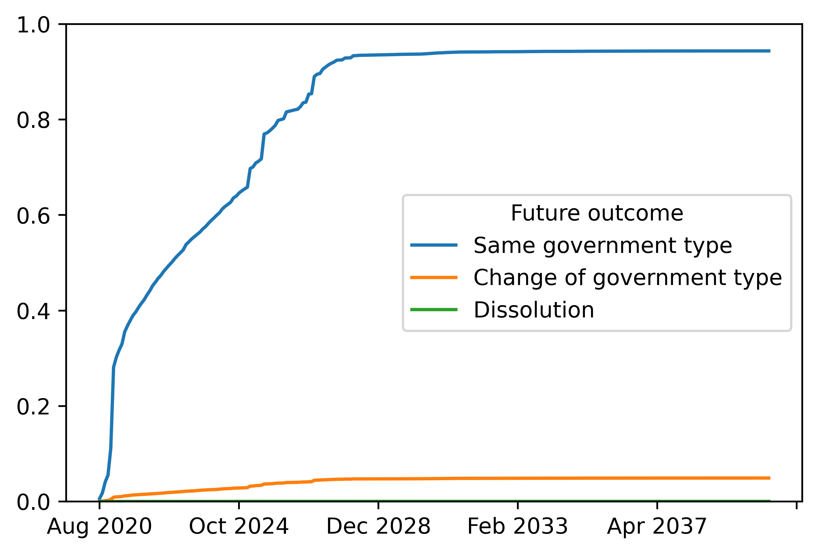
Cumulative Incidence Function¶

It is often of interest to obtain the Cumulative Incidence Function (CIF). The CIF is the probability of a specific type of terminal event on or before any given time period defined as \(Pr(T_i\leq t,D_i=d|X_{i})\). We omit \(\tau\) here for conciseness. The CIF is obtained using the forecasts from LGBSurvivalModeler and LGBExitModeler using the relationship

\[\begin{split}Pr(T_i\leq t,D_i=d|X_{i})&=\sum_{l=T_{i0}+1}^{t}Pr(D_i=d|T_i=l,X_{i})Pr(T_i= l|X_{i})\textrm{, where}\\ Pr(T_i=l|X_{i})&=Pr(T_i\geq l|X_{i})-Pr(T_i\geq l+1|X_{i}).\end{split}\]

Note, we lose forecasts for the last time period due the differencing in the second line.

# Obtain Pr(T=l)
Pr_T_eq_l_forecasts = survival_modeler_forecasts.iloc[:,:-1] - survival_modeler_forecasts.iloc[:,1:].values

# Obtain the cumulative incidence function
cumulative_incidence_forecasts = exit_modeler_forecasts.iloc[:,:-1].copy()
cumulative_incidence_forecasts = cumulative_incidence_forecasts * DataFrame(repeat(Pr_T_eq_l_forecasts.values, repeats = mdata['outcome'].nunique(), axis = 0)).values
cumulative_incidence_forecasts = cumulative_incidence_forecasts.cumsum(axis = 1)
cumulative_incidence_forecasts

country-leader	Future outcome	Aug 2020	Sep 2020	Oct 2020	…	Jun 2040	Jul 2040	Aug 2040
Afghanistan: Ashraf Ghani	Same government type	0.016218	0.025728	0.035270	…	0.820455	0.820492	0.820493
	Change of government type	0.003902	0.006475	0.008134	…	0.163687	0.163696	0.163697
	Dissolution	0.000010	0.000018	0.000026	…	0.001583	0.001583	0.001583
Albania: Rama	Same government type	0.007645	0.014763	0.022883	…	0.938432	0.938476	0.938518
	Change of government type	0.000160	0.000368	0.000698	…	0.045388	0.045400	0.045413
	Dissolution	0.000001	0.000004	0.000007	…	0.000162	0.000162	0.000162
…	…	…	…	…	…	…	…	…
Zambia: Lungu	Same government type	0.006584	0.011123	0.019110	…	0.914390	0.915102	0.915335
	Change of government type	0.000247	0.000377	0.000794	…	0.071899	0.072161	0.072226
	Dissolution	0.000002	0.000003	0.000006	…	0.000178	0.000178	0.000178
Zimbabwe: Mnangagwa	Same government type	0.006362	0.010205	0.016807	…	0.764461	0.764745	0.764987
	Change of government type	0.000364	0.000985	0.001606	…	0.170554	0.170658	0.170798
	Dissolution	0.000002	0.000005	0.000009	…	0.000389	0.000389	0.000389

# Plot cumulative incidence function
plotdf = cumulative_incidence_forecasts.loc["USA: Trump",:].transpose()
plt.figure(dpi=512)
plotdf.plot(ax = plt.gca())
plt.ylim(bottom=0,top=1)

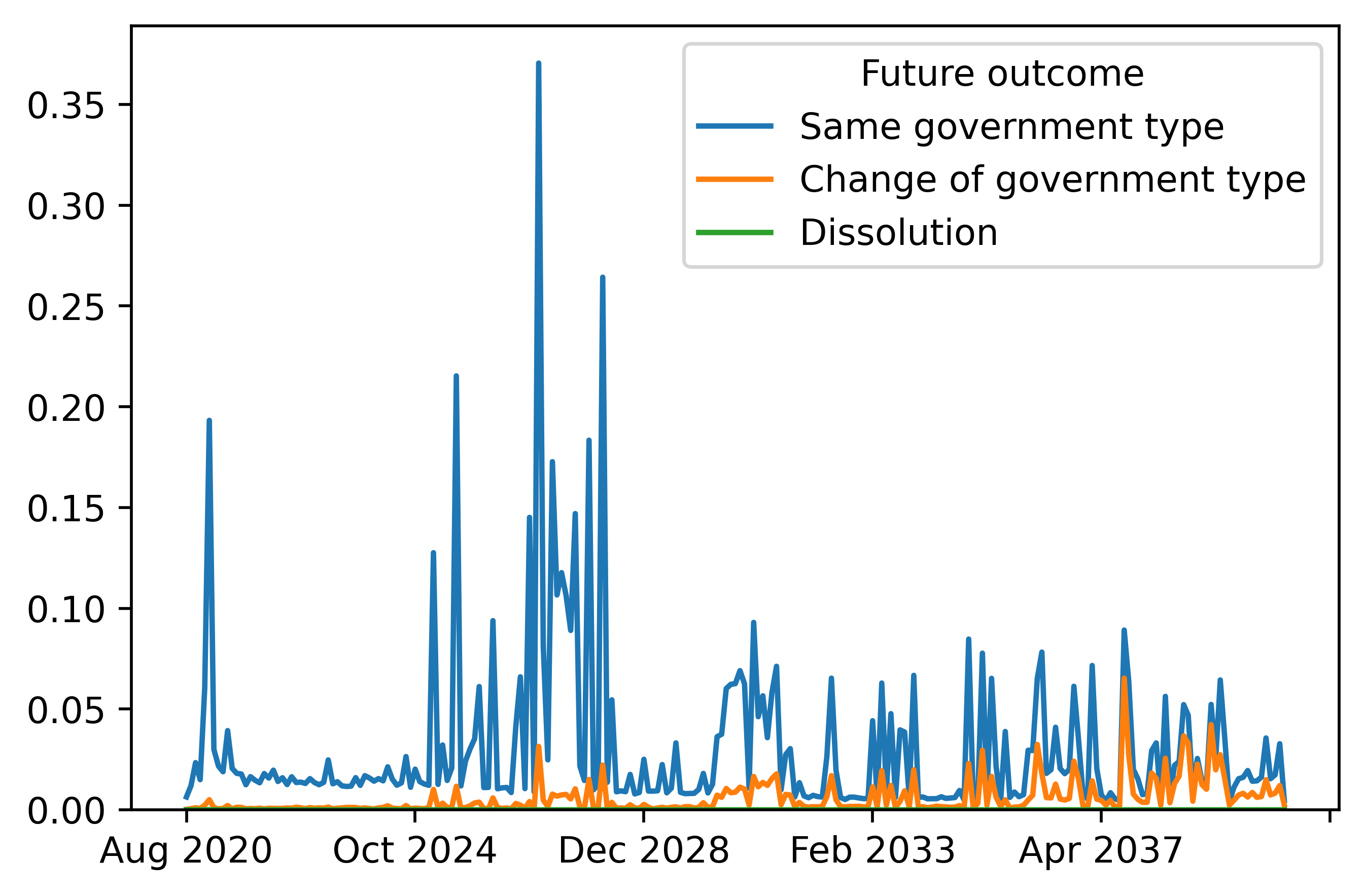
Cause-specific hazard¶

We can also obtain the cause-specific hazard. The cause-specific hazard is the probability of a certain terminal event occuring that time period given that the individual has survived up to the current time period. It is defined as \(Pr(T_i=t,D_i=d|T_i\geq t,X_{i})\). The relationship is

\[Pr(T_i=t,D_i=d|T_i\geq t,X_{i})=\frac{Pr(D_i=d|T_i=t,X_{i})\cdot Pr(T_i=t|X_{i})}{Pr(T_i\geq t|X_{i})}.\]

# Obtain the cause-specific hazard probability forecasts
cause_hazard_forecasts = exit_modeler_forecasts.iloc[:,:-1].copy()
cause_hazard_forecasts = cause_hazard_forecasts * DataFrame(repeat(Pr_T_eq_l_forecasts.values, repeats = mdata['outcome'].nunique(), axis = 0)).values
cause_hazard_forecasts = cause_hazard_forecasts / DataFrame(repeat(survival_modeler_forecasts.iloc[:,:-1].values, repeats = mdata['outcome'].nunique(), axis = 0)).values
cause_hazard_forecasts

country-leader	Future outcome	Aug 2020	Sep 2020	…	Jul 2040	Aug 2040
Afghanistan: Ashraf Ghani	Same government type	0.016447	0.009846	…	1.156903e-01	5.196113e-03
	Change of government type	0.003958	0.002663	…	3.000035e-02	1.463861e-03
	Dissolution	0.000010	0.000009	…	1.312098e-16	6.142482e-18
Albania: Rama	Same government type	0.007704	0.007230	…	5.365918e-03	5.076773e-03
	Change of government type	0.000161	0.000211	…	1.391469e-03	1.612481e-03
	Dissolution	0.000001	0.000002	…	6.085742e-18	6.372296e-18
…	…	…	…	…	…	…
Zambia: Lungu	Same government type	0.006630	0.004602	…	1.065741e-01	4.071534e-02
	Change of government type	0.000248	0.000133	…	3.911648e-02	1.147042e-02
	Dissolution	0.000002	0.000001	…	1.438005e-16	4.813083e-17
Zimbabwe: Mnangagwa	Same government type	0.006406	0.003896	…	4.921725e-03	4.215764e-03
	Change of government type	0.000367	0.000629	…	1.806447e-03	2.444209e-03
	Dissolution	0.000002	0.000003	…	6.640887e-18	7.149276e-18

# Plot cause-specific hazard probabilities
plotdf = cause_hazard_forecasts.loc["USA: Trump",:].transpose()
plt.figure(dpi=512)
plotdf.plot(ax = plt.gca())
plt.ylim(bottom=0)

References¶

Schmid, M., & Berger, M. (2020) Competing risks analysis for discrete time‐to‐event data. Wiley Interdisciplinary Reviews: Computational Statistics, e1529.